Applier Examples¶

To honor the similarities of HUBDC with RIOS, we replicate the examples known from RIOS, and add some more HUBDC specific examples.

Simple Example (explained in detail)¶

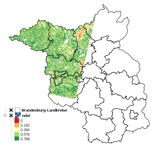
Use the Red and NIR bands of the Landsat LT51940232010189KIS01 scene to calculate the Normalized Difference Vegetation Index (NDVI). Additionally, use the BrandenburgDistricts vector polygon layer to mask the result.

"""
Calculate the Normalized Difference Vegetation Index (NDVI) for a Landsat 5 scene.
Mask the resulting image to the shape of Brandenburg (a federated state of Germany).
"""

import tempfile
import os
import numpy
from hubdc.applier import *
from hubdc.testdata import LT51940232010189KIS01, BrandenburgDistricts

# Set up input and output filenames.
applier = Applier()
applier.inputRaster.setRaster(key='red', value=ApplierInputRaster(filename=LT51940232010189KIS01.red))
applier.inputRaster.setRaster(key='nir', value=ApplierInputRaster(filename=LT51940232010189KIS01.nir))
applier.inputVector.setVector(key='brandenburg', value=ApplierInputVector(filename=BrandenburgDistricts.shp))
applier.outputRaster.setRaster(key='ndvi', value=ApplierOutputRaster(filename=os.path.join(tempfile.gettempdir(), 'ndvi.img')))

# Set up the operator to be applied
class NDVIOperator(ApplierOperator):
    def ufunc(operator):

        # read image data
        red = operator.inputRaster.raster(key='red').array()
        nir = operator.inputRaster.raster(key='nir').array()
        brandenburg = operator.inputVector.vector(key='brandenburg').array(initValue=0, burnValue=1)

        # calculate ndvi, clip to 0-1 and mask Brandenburg
        ndvi = numpy.float32(nir-red)/(nir+red)
        np.clip(ndvi, 0, 1, out=ndvi)
        ndvi[brandenburg==0] = 0

        # write ndvi data
        operator.outputRaster.raster(key='ndvi').setArray(array=ndvi)
        operator.outputRaster.raster(key='ndvi').setNoDataValue(0)

# Apply the operator to the inputs, creating the outputs.
applier.apply(operatorType=NDVIOperator)
print(applier.outputRaster.raster(key='ndvi').filename())

# Python prints something like:
# >>> c:\users\USER\appdata\local\temp\ndvi.img

The result is stored in the file called ndvi.img stored in the user tempdir.

HUB-Datacube Applier programs are usually structured in the following way:

Initialize the Applier
```
applier = Applier()
```
Assigning raster inputs …
```
applier.inputRaster.setRaster(key='image1', value=ApplierInputRaster(filename=LT51940232010189KIS01.swir1))
applier.inputRaster.setRaster(key='image2', value=ApplierInputRaster(filename=LT51940232010189KIS01.swir2))
```
… vector inputs …
```
applier.inputVector.setVector(key='brandenburg', value=ApplierInputVector(filename=BrandenburgDistricts.shp))
```
… and raster outputs
```
applier.outputRaster.setRaster(key='outimage', value=ApplierOutputRaster(filename=os.path.join(tempfile.gettempdir(), 'outimage.img')))
```
Note that all input and output datasets are set using different members of the applier object:

applier.inputRaster is an ApplierInputRasterGroup object, which is a container for ApplierInputRaster objects

applier.inputVector is an ApplierInputVectorGroup object, which is a container for ApplierInputVector objects

applier.outputRaster is an ApplierOutputRasterGroup object, which is a container for ApplierOutputRaster objects
Implement an operator class derived from ApplierOperator and overwriting the ufunc method
```
class NDVIOperator(ApplierOperator):
    def ufunc(operator):
        ...
```
The ufunc method is usually structured into the sections:
1. read data into numpy arrays
  # read image data red = operator.inputRaster.raster(key='red').array() nir = operator.inputRaster.raster(key='nir').array() brandenburg = operator.inputVector.vector(key='brandenburg').array(initValue=0, burnValue=1, dtype=numpy.uint8)
  Note that all input datasets are access using different members of the operator object:
  
  operator.inputRaster is identical to applier.inputRaster and used to access previously defined ApplierInputRaster objects, which can be used to read raster data, see array()
  
  operator.inputVector is identical to applier.inputVector and is used to access previously defined ApplierInputVector objects, which can be used to read and rasterize vector data, see array()
  
  Also note that input data is presented as numpy arrays, of the datatype corresponding to that in the raster files. It is the responsibility of the user to manage all conversions of datatypes.
  
  All blocks of data are 3-d numpy arrays. The first dimension corresponds to the number of layers in the image file, and will be present even when there is only one layer. The second and third dimensions represent the spatial extent (ysize, xsize) of the image block.
2. data processing
  # calculate ndvi and mask Brandenburg ndvi = numpy.float32(nir-red)/(nir+red) ...
3. write output data (and metadata - not shown here)
  # write ndvi data operator.outputRaster.raster(key='ndvi').setImageArray(array=ndvi) ...
  Note that output raster datasets are access using the operator.outputRaster, which is identical to applier.outputRaster and used to access previously defined ApplierOutputRaster objects, which can be used to write output numpy arrays, see setArray().
  
  The datatype of the output files will be inferred from the datatype of the given numpy arrays. So, to control the datatype of the output file, use for example the numpy.astype function to control the datatype of the output arrays.

Manage Metadata Example¶

You can read metadata from input and write metadata to output datasets

This simple example reads the wavelength information from the ENVI metadata domain of an input dataset and passes it to an output dataset:

def ufunc(operator):

    # copy raster data
    array = operator.inputRaster.raster(key='image').imageArray()
    operator.outputRaster.raster(key='outimage').setImageArray(array=array)

    # copy ENVI/wavelength metadata
    wavelength = operator.inputRaster.raster(key='image').metadataItem(key='wavelength', domain='ENVI')
    operator.outputRaster.raster(key='outimage').setMetadataItem(key='wavelength', value=wavelength, domain='ENVI')

See metadataItem() and setMetadataItem() for more details.

For more information on the GDAL Data and Metadata Model see the GDAL documentation.

For more information on the ENVI Metadata Model see The ENVI Header Format

Passing Other Data Example¶

Use additional arguments for passing other data into the operator user function, apart from the raster data itself. This is obviously useful for passing parameters into the processing.

Use the return statement to pass information out again.

A simple example, using it to pass in a single parameter, might be a program to multiply an input raster by a scale value and add an offset:

class ScaleOperator(ApplierOperator):
    def ufunc(operator, scale, offset):
        array = operator.inputRaster.raster(key='image').imageArray()
        scaled = array * scale + offset
        operator.outputRaster.raster(key='outimage').setImageArray(array=scaled)

applier.apply(operatorType=Scaleperator, scale=1, offset=0)

An example of using the return statement to accumulate information across blocks might be a program to calculate some statistic (e.g. the mean) across the whole raster:

class MeanOperator(ApplierOperator):
    def ufunc(operator):
        array = operator.inputRaster.raster(key='image').imageArray()
        blockTotal = img.sum()
        blockCount = img.size
        return blockTotal, blockCount

results = applier.apply(operatorType=MeanOperator)

total, count = 0., 0
for blockTotal, blockCount in results:
    total += blockTotal
    count += blockCount

print('Average value = ', total / count)

The total and count values are calculated from the list of blockTotal and blockCount values returned by the apply() method.

The values could be accumulated between blocks, as looping sequentially over all blocks in the image, but this approach would fail if the applier is used with multiprocessing enabled.

Of course, there already exist superior ways of calculating the mean value of an image, but the point about using the applier to do something like this would be that: a) opening the input rasters is taken care of; and b) it takes up very little memory, as only small blocks are in memory at one time. The same mechanism can be used to do more specialized calculations across the images.

Note that there are no output rasters from the last example - this is perfectly valid.

Controlling the Reference Pixel Grid Example¶

Use setProjection(), setResolution(), and setExtent() to explicitely control the grid projection, resolution and extent:

applier.controls.setProjection(projection=Projection('PROJCS["UTM_Zone_33N",GEOGCS["GCS_WGS_1984",DATUM["WGS_1984",SPHEROID["WGS_84",6378137.0,298.257223563]],PRIMEM["Greenwich",0.0],UNIT["Degree",0.0174532925199433]],PROJECTION["Transverse_Mercator"],PARAMETER["False_Easting",500000.0],PARAMETER["False_Northing",0.0],PARAMETER["Central_Meridian",15.0],PARAMETER["Scale_Factor",0.9996],PARAMETER["Latitude_Of_Origin",0.0],UNIT["Meter",1]]'))
applier.controls.setExtent(extent=Extent(xmin=4400000, xmax=450000, ymin=3100000, ymax=3200000)
applier.controls.setResolution(resolution=Resolution(x=30, y=30)

Other Controls¶

Other controls which can be manipulated are detailed in the ApplierControls class.

Arbitrary Numbers of Input (and Output) Files Example¶

As mentioned before, the applier members applier.inputRaster, applier.inputVector and applier.outputRaster are container objects of type ApplierInputRasterGroup, ApplierInputVectorGroup and ApplierOutputRasterGroup respectively.

These containers are used to store ApplierInputRaster, ApplierInputVector and ApplierOutputRaster objects respectively.

Furthermore, a container can store other containers of the same type, which enables the creation of more complex, nested dataset structures. This makes it possible to represent naming structures comparable to those on the users file system.

An example: given a small Landsat archive of 8 scenes in 4 footprints stored on the file system structured by path/row/scene. Let assume, we are only interested in the CFMask datasets:

C:\landsat\
    194\
        023\
            LC81940232015235LGN00\
                LC81940232015235LGN00_cfmask.img
                 ...
            LE71940232015275NSG00\
                LE71940232015275NSG00_cfmask.img
                ...
            LT41940231990126XXX05\
                LT41940231990126XXX05_cfmask.img
                ...
            LT51940232010189KIS01\
                LT51940232010189KIS01_cfmask.img
                ...
    194\
        024\
            LC81940242015235LGN00\
                LC81940242015235LGN00_cfmask.img
                ...
            LE71940242015275NSG00\
                LE71940242015275NSG00_cfmask.img
                ...
            LT41940241990126XXX03\
                LT41940241990126XXX03_cfmask.img
                ...
            LT51940242010189KIS01\
                LT51940242010189KIS01_cfmask.img
                ...

The CFMask datasets can be inserted manually (preserving the file structure) as follows:

landsat = applier.inputRaster.setGroup('landsat', value=ApplierInputRasterGroup())
path194 = landsat.setGroup('194', value=ApplierInputRasterGroup())
row023 = path194.setGroup(key='023', value=ApplierInputRasterGroup())
row024 = path194.setGroup(key='024', value=ApplierInputRasterGroup())

row023.setRaster(key='LC81940232015235LGN00_cfmask', value=ApplierInputRaster(filename=r'C:\landsat\194\023\LC81940232015235LGN00\LC81940232015235LGN00_cfmask.img'))
...
row024.setRaster(key='LT51940242010189KIS01_cfmask', value=ApplierInputRaster(filename=r'C:\landsat\194\023\LT51940242010189KIS01\LT51940242010189KIS01_cfmask.img'))

The same result can be achieved using the fromFolder() auxilliary method, which takes a folder and searches recursively for all raster matching the given extensions and passes a (optional) ufunc filter function:

ufunc = lambda root, basename, extension: basename.endswith('cfmask'))
applier.inputRaster.setGroup(key='landsat', value=ApplierInputRasterGroup.fromFolder(folder=r'C:\Work\data\gms\landsat',
                                                                                     extensions=['.img'],
                                                                                     ufunc=ufunc)

Inside the operator ufunc, individual datasets can then be accessed as follows:

def ufunc(operator):
    # access individual dataset
    cfmask = operator.inputRaster.group(key='landsat').group(key='194').group(key='023').group(key='LC81940232015235LGN00').raster(key='LC81940232015235LGN00_cfmask')
    array = cfmask.imageArray()

Or as a shortcut to this it is possible to also use key concatenation like so:

cfmask = operator.inputRaster.raster(key='landsat/194/023/LC81940232015235LGN00/LC81940232015235LGN00_cfmask')

To visit all datasets, the structure can be iterated in accordance to how it was created, from landsat, over pathes, over rows, over scenes, to the cfmask rasters:

def ufunc(operator):
    # iterate over all datasets
    landsat = operator.inputRaster.group(key='landsat')
    for path in landsat.groups():
        for row in path.groups():
            for scene in row.groups():
                cfmask = scene.findRaster(ufunc=lambda key, raster: key.endswith('cfmask'))
                array = cfmask.imageArray()

The rasters can also be flat iterated, ignoring the group structure completely:

def ufunc(operator):
    # flat iterate over all datasets
    for cfmask in operator.inputRaster.flatRasters():
        array = cfmask.imageArray()

Filters and Overlap Example¶

Because the applier operates on a per block basis, care must be taken to set the overlap correctly when working with filters. The overlap keyword must be consistently set when using input raster reading methods ( imageArray(), bandArray(), fractionArray()), input vector reading methods ( imageArray() fractionArray()), and output raster writing method ( setImageArray()).

Here is a simple convolution filter example:

import tempfile
import os
from scipy.ndimage import uniform_filter

from hubdc.applier import *
from hubdc.testdata import LT51940232010189KIS01

applier = Applier()
applier.inputRaster.setRaster(key='image', value=ApplierInputRaster(filename=LT51940232010189KIS01.band3))
applier.outputRaster.setRaster(key='outimage', value=ApplierOutputRaster(filename=os.path.join(tempfile.gettempdir(), 'smoothed.img')))

class SmoothOperator(ApplierOperator):
    def ufunc(operator):

        # does a spatial 11x11 uniform filter.
        # Note: for a 3x3 the overlap is 1, 5x5 overlap is 2, ..., 11x11 overlap is 5, etc
        overlap = 5
        array = operator.inputRaster.raster(key='image').imageArray(overlap=overlap)
        arraySmoothed = uniform_filter(array, size=11, mode='constant')
        operator.outputRaster.raster(key='outimage').setImageArray(array=arraySmoothed, overlap=overlap)

applier.apply(operatorType=SmoothOperator)

Many other Scipy filters are also available and can be used in a similar way.

Categorical Raster Inputs Example¶

On-the-fly resampling and reprojection of input rasters into the reference pixel grid is one key feature of the applier. However, for categorical raster inputs, this default behaviour can be insufficient in terms of information content preservation, even if the resampling algorithm is carefully choosen.

For example, if the goal is to process a categorical raster, where different categories are coded with unique ids, standard resampling algorithms will not be able to preserve the information content.

Sometimes it is sufficient to use the gdal.GRA_Mode algorithms, but in general it is not. To resample a categorical raster into a target pixel grid with a different resolution usually implies that the categorical information must be aggregated into pixel fraction, one for each category.

In the following example a Landsat CFMask image at 30 m is resampled into 250 m, resulting in a category fractions. The categories are: 0 is clear land, 1 is clear water, 2 is cloud shadow, 3 is ice or snow, 4 is cloud and 255 is the background. Use fractionArray() to achieve this:

cfmaskFractions250m = self.inputRaster.raster('cfmask30m').fractionArray(categories=[0, 1, 2, 3, 4, 255])

Categories at 250 m can then be calculated from the aggregated fractions:

cfmask250m = numpy.array([0, 1, 2, 4, 255])[cfmaskFractions250m.argmax(axis=0)]

Vector Inputs Example¶

Vector layers can be included into the processing:

applier = Applier()
applier.inputVector.setVector(key='vector', value=ApplierInputVector(filename=myShapefile))

Like any input raster file, vector layers can be accessed via the operator object inside the user function:

def ufunc(operator):
    vector = operator.inputVector.vector(key='vector')

Use imageArray() to get a rasterized version of the vector layer. The rasterization is a binary mask by default, that is initialized with 0 and all pixels covered by features are filled (burned) with a value of 1:

array = vector.imageArray()

This behaviour can be altered using the initValue and burnValue keywords:

array = vector.imageArray(initValue=0, burnValue=1)

Instead of a constant burn value, a burn attribute can be set by using the burnAttribute keyword:

array = vector.imageArray(burnAttribute='ID')

Use the filterSQL keyword to set an attribute query string in form of a SQL WHERE clause. Only features for which the query evaluates as true will be returned:

sqlWhere = "Name = 'Vegetation'"
array = vector.imageArray(filterSQL=sqlWhere)

Categorical Vector Inputs Example¶

In some situations it may be insufficient to simply burn a value or attribute value (i.e. categories) onto the target reference pixel grid. Depending on the detailedness of the vector shapes (i.e. scale of digitization), a simple burn or not burn decision may greatly degrade the information content if the target resolution (i.e. scale of rasterization) is much coarser.

In this case it would be desirable to rasterize the categories at the scale of digitization and afterwards aggregate this categorical information into pixel fraction, one for each category.

Take for example a vector layer with an attribute CLASS_ID coding features as 1 -> Impervious, 2 -> Vegetation, 3 -> Soil and 4 -> Other. To derieve aggregated pixel fractions for Impervious, Vegetation and Soil categories rasterization at 5 m resolution use fractionArray():

def ufunc(operator):
    vector = operator.inputVector.vector(key='vector')
    fractions = self.fractionArray('vector', categories=[1, 2, 3], categoryAttribute='CLASS_ID',
                                   resolution=Resolution(x=5, y=5).

Instaed of explicitly specifying the rasterization resolution, use the oversampling keyword to specify the factor by witch the target resolution should be oversampled. Note that if nothing is specified, an oversampling factor of 10 is used. So for example, if the target resolution is 30 m and rasterization should take place at 5 m resolution, use an oversampling factor of 6 (i.e. 30 m / 5 m = 6):

fractions = self.fractionArray('vector', categories=[1, 2, 3], categoryAttribute='CLASS_ID',
                               oversampling=6)

Categories at 30 m can then be calculated from the aggregated fractions:

categories = numpy.array([1, 2, 3])[fractions.argmax(axis=0)]

Parallel Processing Example¶

Each block can be processed on a seperate CPU using Python’s multiprocessing module. Making use of this facility is very easy and is as simple as setting some more options on the applier.controls object , see setNumThreads(). Note, that under Windows you need to use the if __name__ == '__main__': statement:

def ufunc(operator):
    ...

if __name__ == '__main__':

    applier = Applier()
    # ...
    applier.controls.setNumThreads(5)
    applier.apply(ufunc)

Parallel Writing Example¶

It is possible to have multiple writer processes. Using multiple writers (in case of multiple outputs) makes sense, because writing outputs is not only limitted by the hard drive, but also by data compression and other CPU intense overhead. Making use of this facility is also very easy and is as simple as setting some more options on the applier.controls object , see setNumWriter():

applier.controls.setNumWriter(5)

Setting GDAL Options Example¶

Via the applier.controls object you can set various GDAL config options (e.g. setGDALCacheMax()) to handle the trade of between processing times and memory consumption:

applier = Applier()
applier.controls.setGDALCacheMax(bytes=1000*2**20)
applier.controls.setGDALSwathSize(bytes=1000*2**20)
applier.controls.setGDALDisableReadDirOnOpen(disable=True)
applier.controls.setGDALMaxDatasetPoolSize(nfiles=1000)